Functions for lookup of data

These functions perform a lookup on a data range using the provided value and return the result.

ADDRESS

Returns the cell reference for the given row and column, or the current cell.

If you do not specify a row and column, the current cell is used.

This function is useful for dynamically referring to specific cells in models, which is helpful in generating references in models or reports.

ADDRESS(row, column)

Examples:
ADDRESS(2, 3) = "C2"
ADDRESS() = "C2" (current cell)

ARRAY ❖ XLReporting

Returns multiple individual values (including any empty values) as a data array or cell range.

You can use this function to place multiple individual values or cell references into one single data array, which you can then (as example) push into a function that expects a single array or cell range as parameter. Empty values are retained in-place in the resulting data array.

This function is useful for building structured data sets from scattered inputs, which is ideal for data consolidation or passing grouped inputs into other functions.

ARRAY(data, data, ..)

Examples:
ARRAY(2, 3) = [2,3]
SUMIF(ARRAY(A1, A10, A20), .., ..)

CELL

Returns the type of value in the given data. Similar to the TYPE function.

This function is useful for validating and categorizing data types in financial models, ensuring consistency across fields.

CELL(data)

The function can return these values:
array   = a data array or cell range
blank   = the following values are considered blank: absent data, empty string "", a single space " ", a "0" text, and a 0 number
error   = a formula error
period  = a period YYYY-MM
date    = a date YYYY-MM-DD
number  = a numerical value
boolean = a boolean value
email   = an email address
phone   = a phone number
url     = a website URL
wrap    = a JSON-formatted text (see WRAP function)
text    = a text string

Example:
CELL(123) = "number"
CELL(A3) = "text"

CELLRANGE ❖ XLReporting

Returns an array with the given cell values, arrays or cell ranges. This function only works on the default sheet (the first or only sheet in the model). Using INDEX you can extract individual values from the array. You can specifiy multiple ranges.

This function is useful for combining multiple value sources into one array, especially for use with filters, lookups, or aggregations.

CELLRANGE(data, data, ..)

Example:
CELLRANGE(A1:A3, B5, C10:C12)

CELLS

Returns the number of cells in the given cell range or data array.

This function is useful for validating the size of data sets, which is ideal in error checking or dynamic formula building.

This function is an alias for the TYPE function and thus identical.

CELLS(data)

Example:
CELLS(A1:C4) = 12

CELLVALUE ❖ XLReporting

Returns the value in the cell with the given cell reference. You can optionally provide the sheet name (as text), else the default sheet (the first or only sheet in the model) will be used. You can only reference one single cell.

This is only relevant in models and enables you to obtain the value in a cell by passing a dynamic text reference to that cell. This enables you to dynamically calculate the reference to a cell within a formula without having to change the formula itself.

This function is useful for indirect referencing in models, when the target cell varies based on user input or formula logic.

IMPORTANT: this function requires that the cell reference and sheet name is given as quoted text strings, for example CELLVALUE("A1", "Sheet1"). This is intentionally different from most other functions because CELLVALUE references a cell by means of a text string.

Please be aware that the sheet and cell references made via CELLVALUE are not adjusted when sheets are renamed and/or rows or columns are inserted or deleted.

CELLVALUE(cell, sheet)

Examples:
CELLVALUE("C2") = 25
CELLVALUE("C2", "Sheet1") = 25

CHOOSE

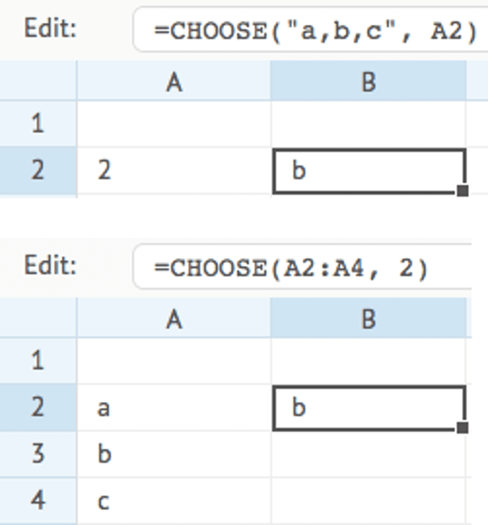
Returns a single value, or range of values, from the given cell range, list of values, or data array, based on the given index, and optional number of items.

If you omit number, a single value will be returned, which is similar to the INDEX function.

If you provide number, a range of values will be returned for the number of items (even if you provide 1). You pass that range of values directly into other functions that expect a cell range or data array.

This function is useful for extracting values from fixed lists or options, such as pricing tiers or scenario selections.

CHOOSE(data, index, number)

Examples:

COLUMNS

Returns the number of columns in the given cell range or data array. The range must contain only one row.

This function is useful for data structure validation or defining dynamic column-based calculations in models.

COLUMNS(data)

Example:
COLUMNS(A1:E1) = 5

COMPARE ❖ XLReporting

Compares the items in the 2 given cell ranges, data arrays, or comma-delimited list of values, and returns the outcome defined by the type parameter. Both ranges need to have the same number of items, and have the same sort order of items. The comparison is case-sensitive.

The optional names parameter defines the field names for each of the items, and can either be a cell range or a comma-delimited list of names. This is only applicable to types 2 and 3.

This function is useful for audit trails, version comparisons, or validating whether imported data has changed.

The purpose of this function is to identify the differences between 2 ranges, for example between multiple edited items against their original items. If you only want to check whether items exist in both ranges, you can use the EXIST function instead.

COMPARE(data, range, type, names)

type:
0 = returns true if the items in both ranges are the same, else returns false (default)
1 = returns the number of items that deviate between both ranges
2 = returns the deviating items as a comma-delimited list
3 = returns each deviating item and its compared item as a comma-delimited list

Examples:
data = "apple,pear,banana"
COMPARE(data, "apple,pear,orange", 1) = 1
COMPARE(data, "apple,pear,orange", 2) = "banana"
COMPARE(data, "apple,pear,orange", 3) = "banana (orange)"

DISTINCT ❖ XLReporting

Returns a sorted list with distinct items that occur in the given cell range, data array, or comma-delimited list of values. You can also use this function to ensure that reports and queries retrieve detailed data for each distinct value in this field, rather than aggregated.

This function is useful for eliminating duplicates, which is ideal for building filters, drop-downs, or generating distinct keys in reports.

DISTINCT(data)

Example:
data = "a,a,b,a,c,b,c,b,a"
DISTINCT(data) = "a,b,c"

EXIST ❖ XLReporting

Checks that items exist in both cell ranges, data arrays, or comma-delimited list of values. The ranges may have different number of items, and different sort order of items. The comparison is case-sensitive.

The purpose of this function is to check whether items exist in both ranges. If you want to compare the items in detail, you can use the COMPARE function instead.

This function is useful for validating completeness (e.g. all required accounts present), or identifying unmatched values across data sets.

EXIST(data, range, type)

type:
0 = returns true if at least 1 item in "data" exist in "values", else returns false (default)
1 = returns true if ALL items in "data" exist in "values", else returns false
2 = returns true if "data" and "values" contain the exact same items, else returns false

Examples:
data = "apple,pear,banana"
EXIST(data, "apple,pear,orange,banana") = true
EXIST(data, "apple,pear,orange,banana", 1) = true
EXIST(data, "apple,pear,orange,banana", 2) = false

EXTRACT ❖ XLReporting

Returns the value or text that resides between the given key and endkey. This function is useful to extract words from texts, or to extract values from within HTML or XML tags.

This function is useful for parsing structured text fields such as comments, notes, XML/HTML snippets, or tagged descriptions.

EXTRACT(data, key, endkey)

Example:
data = "<product>coffee</product> "
EXTRACT(data, "<product>", "</product>") = "coffee"

FILTER

Returns a filtered list with items in the given cell range or data array that meet the given condition. The condition can either be a single value if you just want to compare against that value, or an expression with an operator and value, within quotes (e.g. ">10").

The data parameter is the range of which you want to return the filtered items that meet the condition. If you want to return the items of a range other than data, you can optionally provide the range parameter. You can omit range if it is the same as the data range. Using the optional sort parameter you can sort the list.

This function is similar to the well-known functions SUMIF and COUNTIF, but rather than returning the sum or count of matching items, it returns a filtered (and optionally sorted) list of items.

This function is useful for returning lists of records meeting criteria, like overdue invoices or transactions above a threshold, which is ideal for dashboards or audit trails.

FILTER(data, condition, range, sort)

Examples:
FILTER(A2:A9, ">1000") = "1100,2002,1090"
FILTER(A2:A9, ">1000", A2:A9, 1) = "1090,1100,2002"

FIND

Returns the starting position of a given text string (the key parameter) within another text string (the data parameter).

This function is useful for locating keywords in descriptions, labels, or other semi-structured text fields.

FIND(data, key)

Example:
data = "this text"
FIND(data, "tex") = 6

FIRSTVALUE ❖ XLReporting

Returns the first non-blank and non-zero value in the given cell range of data array. You may specific multiple ranges.

This function is useful for extracting the earliest relevant value in scenarios such as forecast assumptions or progressive account balances.

FIRSTVALUE(data, data, ..)

Example:
FIRSTVALUE("", "a", "", "b", "") = "a"

HLOOKUP

Looks up the given key value in the given horizontal cell range or data array (data), and returns the value in the same column in the second horizontal cell range or data array (range).

The lookup will always try an exact match on the key value, and return an empty text when no exact match is found. If you want to find the nearest or approximate match when no exact match is found, you need to set the type parameter.

This function is useful for retrieving values from row-based data tables, such as exchange rates or timeseries.

This function is an alias for the LOOKUP function and thus identical.

HLOOKUP(data, range, key, type)

type:
0 = exact match only (default)
1 = find the next value just after the given key
2 = find the previous value just before the given key
3 = case-insensitive fuzzy match by ignoring all characters other than A-Z and 0-9

Example:

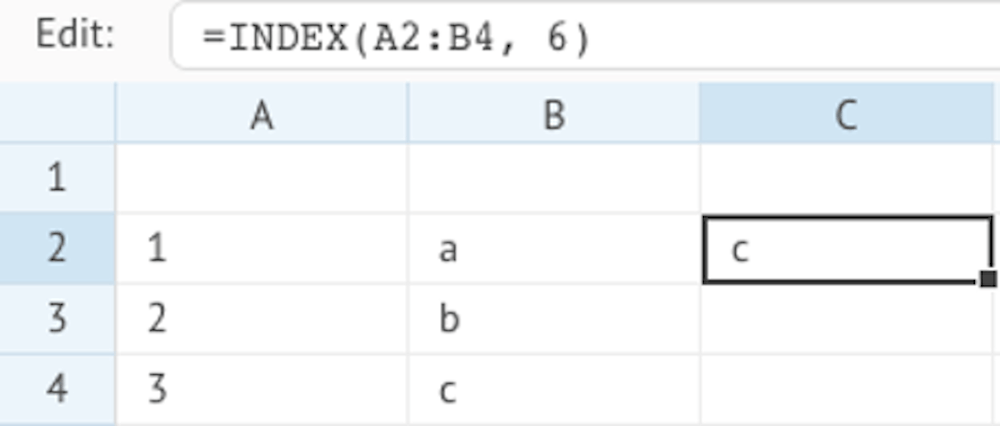
INDEX

Returns a single value from the given cell range or data array, based on the given index. The index is a sequential result of the combined row and column position. For example, a range with 3 rows and 2 columns has 6 indices (3 * 2). The value on row 2 and column 1 has index 3 (1 * 2 + 1), whilst the value on row 3 and column 2 has index 6 (2 * 2 + 2), and so on.

This function is useful for dynamic value extraction in a grid, useful for models and allocation logic.

INDEX(data, index)

Example:

INDIRECT

Returns the value in the cell with the given cell reference, or with the given row and column. You can optionally provide the sheet name (as text), else the default sheet (the first or only sheet in the model) will be used.

This is only relevant in models and enables you to indirectly obtain the value in a cell by setting a dynamic reference to that cell. This enables you to dynamically change the reference to a cell within a formula without having to change the formula itself.

Please be aware that sheet and cell references made via INDIRECT are not adjusted when sheets are renamed and/or rows or columns are inserted or deleted. INDIRECT enables you to set your own dynamic references to cell positions within a model, and is therefore never adjusted.

This function is useful for creating dynamic references that change based on other inputs, enabling flexible model structures.

INDIRECT(cell) or INDIRECT(row, column, sheet)

Examples:
INDIRECT("C2") = 25
INDIRECT(2, 3) = 25
INDIRECT(2, 3, "Sheet1") = 25

JSON ❖ XLReporting

Returns a property value from a JSON-formatted text, based on the given key. You can specify the nodes(s) that represent the property value you want. You can specify nested nodes by a period, e.g. mydata.product.description. You can also specify array positions, e.g. mydata.products.0.id

This function is useful for parsing API responses or JSON-based data integrations in financial workflows.

JSON(data, key)

Example:
data = {"mydata":{"product":{"id":"1","description":"coffee","price":"10"}}}
JSON(data, "mydata.product.description") = "coffee"

LABEL ❖ XLReporting

Returns a text label for the given index by looking it up in the given cell range, data array, or comma-delimited list of values.

This function is useful for generating readable labels from coded values or building user-friendly reports.

LABEL(data, index)

Example:
LABEL("Jan,Feb,Mar", 2) = "Feb"

LASTVALUE ❖ XLReporting

Returns the last non-blank and non-zero value in the given cell range of data array. You may specific multiple ranges.

This function is useful for pulling final or closing values such as ending balances, final status, or latest rates.

LASTVALUE(data, data, ..)

Example:
LASTVALUE("", "a", "", "b", "") = "b"

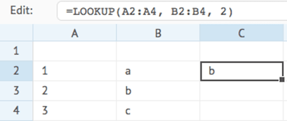
LOOKUP

Looks up the given key value in the given cell range, data array, or comma-delimited list of values (data), and returns the value on the same row in the second cell range, data array, or comma-delimited list of values (range).

The lookup will always try an exact match on the key value, and return an empty text when no exact match is found. If you want to find the nearest or approximate match when no exact match is found, you need to set the type parameter.

This function requires the keys and values to be separated. If the keys and values are combined in one single cell range, data array, or comma-delimited list of values, you can use the SWITCH function instead.

This function is useful for linking data from reference tables like cost centers, product lists, or period assumptions.

LOOKUP(data, range, key, type)

type:
0 = exact match only (default)
1 = find the next value just after the given key
2 = find the previous value just before the given key
3 = case-insensitive fuzzy match by ignoring all characters other than A-Z and 0-9

Example:

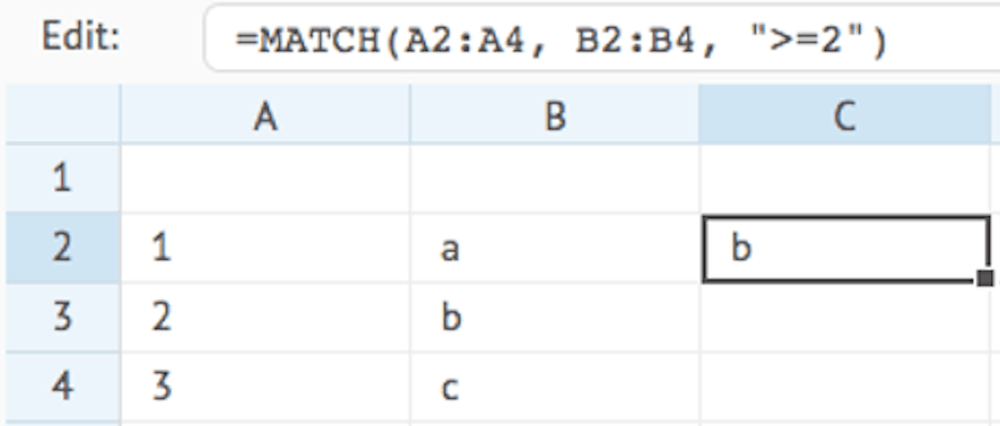
MATCH

Compares each item in the given cell range or data array (data) to a condition, and returns the value on the first row in the second cell range or data array (range) that matches the condition.

This function is useful for conditional lookup where you need to apply filters instead of direct key-based matching

MATCH(data, range, condition)

Example:

OFFSET

Returns a single value from the given cell range or data array, based on the given index. The index is a sequential result of the combined row and column position. For example, a range with 3 rows and 2 columns has 6 indices (3 * 2). The value on row 2 and column 1 has index 3 (1 * 2 + 1), whilst the value on row 3 and column 2 has index 6 (2 * 2 + 2), and so on.

This function is useful for dynamic value extraction in a grid, useful for models and allocation logic.

This function is an alias for the INDEX function and thus identical.

OFFSET(data, index)

Example:
OFFSET(A1:L1, 3) = the value in cell C1

PLAN ❖ XLReporting

Returns the range of values, or the value at the given index, of the given planner. See the PLANNER function below for further reference. No calculation is performed: the function simply returns the value(s), which you can use in your own formula.

If you omit index, the function returns a range with all values.

This function is useful for defining time or allocation patterns to reuse across models, like seasonal distributions.

PLAN(planner, index)

Example:
PLAN("Months", 6) = 1 (the value of given planner index)

The PLAN function works in conjunction with the Cell editor Planner and enables you to define a pattern of values, and use those in formulas.

When you want to use a PLAN function, you first need to define a Cell editor Planner. See the PLANNER function for more details.

PLANNER ❖ XLReporting

Returns a proportion of data using the relative value at the given index of the given planner. The returned value is calculated as follows:

data * (value of given planner index / sum of all planner values)

If the given index does not exist in the planner, the function will use the given ratio (which can be a cell reference, a formula, or a given value) and will return the result of data * ratio.

If neither the index or a ratio exists, the function will return 0 (zero).

This function is useful for distributing amounts across predefined patterns (e.g. 4-4-5, quarterly splits) for accurate planning.

PLANNER(data, planner, index, ratio)

Examples:
PLANNER(1000, "Months", 6)     = 83.33  (1000 * 1 / 12)
PLANNER(1000, "Weeks445", 6)   = 96.15  (1000 * 5 / 52)
PLANNER(1000, "Summmer", 6)    = 111.11 (1000 * 4 / 36)
PLANNER(1000, "", 0, B3/C3)    = 200.00 (1000 * 1 / 10)

The PLANNER function works in conjunction with the Cell editor Planner and enables you to distribute a given value across a range of cells in a model, based on a defined pattern that can be selected by the user. For example, this can be used to divide an given amount over a range of periods, or across products etc.

When you want to use a PLANNER function, you first need to define a Cell editor Planner.

The below example defines 4 patterns for a cell editor: monthly, quarterly, every half year, and a custom pattern:

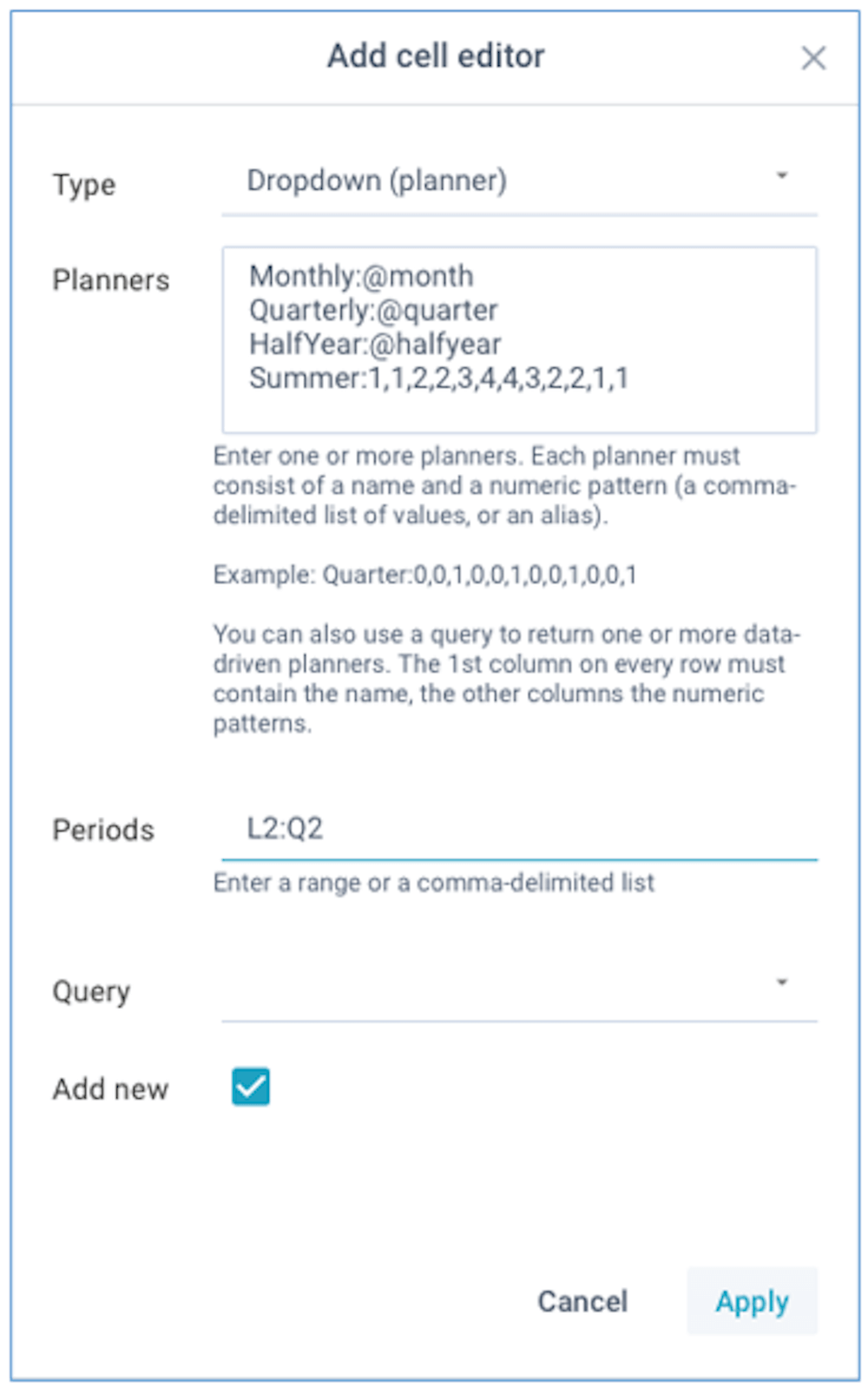
The absolute values of the numeric patterns are irrelevant, what matters is each relative value as a proportion of the sum of all values. You can define as many indices in the patterns as you need.

You can also use one of the below aliases for common patterns:

• @month - every month (1,1,1,1,1,1,1,1,1,1,1,1)
• @quarter - every quarter (0,0,1,0,0,1,0,0,1,0,0,1)
• @soquarter - start of every quarter (1,0,0,1,0,0,1,0,0,1,0,0)
• @halfyear - every half year (0,0,0,0,0,1,0,0,0,0,0,1)
• @sohalfyear - start of every half year (1,0,0,0,0,0,1,0,0,0,0,0)
• @year - every year (0,0,0,0,0,0,0,0,0,0,0,1)
• @soyear - start of every year (1,0,0,0,0,0,0,0,0,0,0,0)
• @period445 - based on 4-4-5 weeks (4,4,5,4,4,5,4,4,5,4,4,5)

In addition to defined static planners, you can also refer to a data query. Your data query can include multiple rows, with each row being treated as a separate planner. The first column on every row needs to contain the planner name, and the other columns need to contain the numeric patterns.

PRETTY ❖ XLReporting

Returns a formatted and easily readable text from the given JSON-formatted text, cell range, data array, or comma-delimited list of values (data), each value prefixed with its associated labels. The labels have to be a comma-delimited list of values.

The result will be a text in the form of "label1=value1, label2=value2, ..." with each value joined with its respective label. Values without associated labels will be ignored.

This function is useful for presenting compact summaries of multi-part values in readable report outputs.

PRETTY(data, labels)

Examples:
PRETTY(A2:A3, "key,value") = "key=abc, value=1000"
PRETTY("abc,1000", "key,value") = "key=abc, value=1000"
PRETTY("{"a":"abc","b":"1000"}", "key,value") = "key=abc, value=1000"

RANK

Returns the rank (the relative position, starting at 1) of a given number within the list of numbers in the given cell range, data array, or comma-delimited list of values. Using the optional type parameter, you can decide if (and how) the list will be sorted.

The function performs an exact match, unless you specify type 2 (nearest match). If no exact match is found, the function will return 0. If you want to find the nearest match, this will automatically sort the list in ascending order.

This function is useful for scoring, benchmarking, or ranking financial metrics within portfolios or business units.

RANK(data, number, type)

type:
0 = ascending sort (default)
1 = descending sort
2 = nearest match in ascending sort
3 = no sort

Example:
data = "200,500,300"
RANK(data, 300, 0) = 2

ROWS

Returns the number of rows in the given cell range or data array. The range must contain only one column.

This function is useful for validating dataset size or controlling loops or dynamic allocations in models.

ROWS(data)

Example:
ROWS(A1:A4) = 4

SEQUENCE

Returns an array of numbers, dates, or periods from the given start for the given number of increments. The returned data has the same structure as a cell range or data array, which enables you to pass this data directly into a dropdown editor or other functions that expect a cell range or data array. You can optionally pass an interval (default is 1). The interval can be positive or negative.

You can also use a text as data, in which case it will be suffixed by a numeric series.

This function automatically determines the type of data and then calls either PERIODRANGE, DATERANGE, or the NUMRANGE function.

This function is useful for automating numeric, date, or period-based lists, which is handy for schedules and simulations.

SEQUENCE(data, number, interval)

Examples:
SEQUENCE(5, 4) = 5, 6, 7, 8
SEQUENCE(5, 4, 10) = 5, 15, 25, 35
SEQUENCE("2019-01", 3, 12) = "2019-01", "2020-01", "2021-01"
SEQUENCE("col", 4) = "col0", "col1", "col2", "col3"

SETWRAP ❖ XLReporting

Updates a specific value within a JSON-formatted text that was created by WRAP. The key is numeric in order of the values passed to WRAP (e.g. 1, 2, 3 etc). Use WRAP to create the JSON-formatted text, or UNWRAP to extract the data again.

This function is useful for modifying structured data passed between components or stored in datasets.

SETWRAP(data, value, key)

Example:
SETWRAP(data, 25, 2)

SWITCH

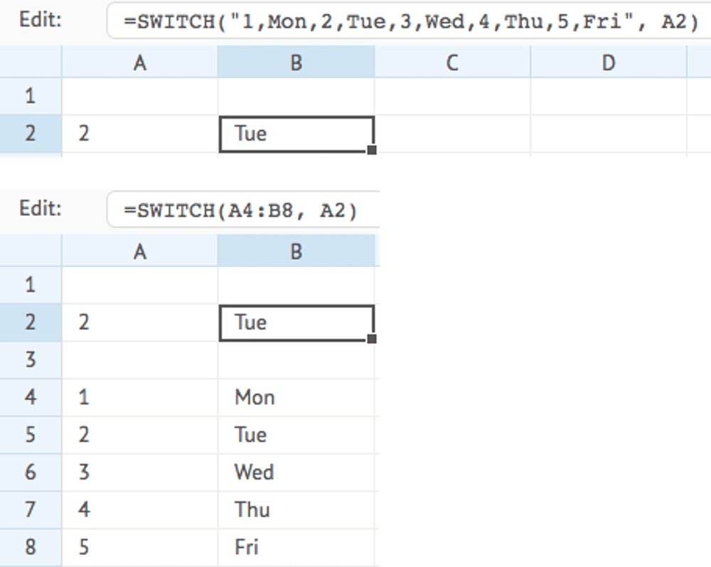
Returns the corresponding value that matches the given key in the given cell range, data array, or comma-delimited list of values. The list must contain the keys and their corresponding values as separate consequtive items. If no value is found, either the key is returned, or an empty value if you set the empty parameter to true.

This function is similar to the LOOKUP function but, instead of separate keys and values, it supports combined keys and values in one single cell range, data array, or comma-delimited list of values.

This function is useful for replacing small lookup tables in formulas, like tax brackets or option selectors.

SWITCH(data, key, empty)

Examples:

TAKE ❖ XLReporting

Returns an array with the given cell values, arrays or cell ranges. Using INDEX you can extract individual values from the array. You may specific multiple ranges.

This function is useful for grouping inputs into arrays for further processing or transformation.

This function is an alias for the CELLRANGE function and thus identical.

TAKE(data, data, ..)

Example:
TAKE(A1:A3, B5, C10:C12)

TYPE

Returns the type of value in the given data. If the optional type parameter is given, returns true if the data matches the expected type.

This function is useful for validating values before calculations or filtering by content type.

TYPE(data, type)

type:
"array"   = a data array or cell range
"blank"   = the following values are considered blank: absent data, empty string "", a single space " ", a "0" text, and a 0 number
"error"   = a formula error
"period"  = a period YYYY-MM
"date"    = a date YYYY-MM-DD
"number"  = a numerical value
"boolean" = a boolean value
"email"   = an email address
"phone"   = a phone number
"url"     = a website URL
"wrap"    = a JSON-formatted text (see WRAP function)
"text"    = a text string

Example:
TYPE(123) = "number"
TYPE(123, "number") = true
CELL(A3) = "text"

UNIQUE

Returns a sorted list with unique items that occur in the given cell range, data array, or comma-delimited list of values.

This function is useful for creating dropdowns or analyzing diversity within a dataset like unique accounts or products.

This function is an alias for the DISTINCT function and thus identical.

UNIQUE(data)

Example:
data = "a,a,b,a,c,b,c,b,a"
UNIQUE(data) = "a,b,c"

UNWRAP ❖ XLReporting

Returns a specific value from a JSON-formatted text that was created by WRAP. The key is numeric in order of the values passed to WRAP (e.g. 1, 2, 3 etc). Use WRAP to create the JSON-formatted text.

This function is useful for unpacking structured or compound values in reporting or integration workflows.

UNWRAP(data, key)

Example:
UNWRAP(data, 2)

VLOOKUP

Looks up the given key value in the given vertical cell range or data array, and returns the value on the same row in the second vertical cell range or data array (range).

The lookup will always try an exact match on the key value, and return an empty text when no exact match is found. If you want to find the nearest or approximate match when no exact match is found, you need to set the type parameter.

This function is useful for matching IDs or codes to descriptive values from lists organized in columns.

This function is an alias for the LOOKUP function and thus identical.

VLOOKUP(data, range, key, type)

type:
0 = exact match only (default)
1 = find the next value just after the given key
2 = find the previous value just before the given key
3 = case-insensitive fuzzy match by ignoring all characters other than A-Z and 0-9

Example:

WEBSERVICE

Returns data from a web service on the Internet or Intranet. Only connections over https:// are allowed.

If the data is returned in JSON format, you can use the key parameter to specify the JSON node(s) that contains the required value(s). You can specify nested nodes by a period, e.g. mydata.product.description. You can also specify array positions, e.g. "mydata.products.[0].id". If you don't specify any node, the entire JSON data will be returned as text and you can use the JSON function to extract the necessary value(s) from that data.

On any data that is returned by this function, you can use other lookup and text functions (e.g. FIND, EXTRACT, LEFT, MID, RIGHT etc) to extract the required value(s).

Please note that the data is being cached for performance reasons. The data will be retrieved from the web service when the formula is first executed, but not refreshed during every subsequent recalculation.

This function is useful for integrating external data (e.g. FX rates, KPIs) into your financial models.

WEBSERVICE(url, key)

Example:
WEBSERVICE("https://api.exchangeratesapi.io/latest", "rates.USD")

WEBVIEW ❖ XLReporting

Views the content of a web page on the Internet or Intranet. You can optionally define the width and height of the window that contains the content.

Please note that for security reasons this is allowed for approved websites only, and only for https:// connections. By default, you can only link to pages on https://www.xlreporting.com. If you want to link to an external website or to your company intranet, please contact us.

This function is useful for embedding reference content, documentation, or contextual dashboards.

WEBVIEW(url, width, height)

Example:
WEBVIEW("https://www.xlreporting.com")

WITHIN ❖ XLReporting

Returns true if the given data falls between any of the given from/to value pairs, else returns false. You can provide any number of values. This function works with numbers, texts, dates, or periods.

This function is useful for range filtering with multiple scenarios like discount brackets or performance bands.

WITHIN(data, from, to, from, to, ..)

Example:
data = 100
WITHIN(data, 120, 140, 80, 110, 30, 40) = true

WRAP ❖ XLReporting

Wraps a given cell range, data array, or list of values into a JSON-formatted text. Ideal for storing complex data into a single value, for example when saving into a data set column. Each value is given a sequential numeric key starting at 1 (e.g. 1, 2, 3 etc) in order of the values passed. Use UNWRAP to extract the data again, or SETWRAP to update a specific value. You may specific multiple ranges.

Please note that each parameter is treated as one value. If you provide a cell range with multiple cells, the cell values will be concatenated into one single value in the JSON-formatted text. Alternatively, you can provide each cell reference as a separate parameter.

This function is useful for compactly storing or transferring multiple values as one, useful in custom exports or field packing.

WRAP(data, data, ..)

Examples:
WRAP(A3:B3)
WRAP(A3, B3, C3)

XLOOKUP

Looks up the given key value in the given cell range or data array (data), and returns the value on the same row in the second cell range or data array (range).

The lookup will always try an exact match on the key value, and return an empty text (or the optional notfound value) when no exact match is found. If you want to find the nearest or approximate match when no exact match is found, you need to set the type parameter.

This function is useful for robust lookups that default gracefully when data is missing, which is ideal in user-facing reports.

This function is an alias for the LOOKUP function and thus identical.

XLOOKUP(data, range, key, notfound, type)

type:
0 = exact match only (default)
1 = find the next value just after the given key
2 = find the previous value just before the given key
3 = case-insensitive fuzzy match by ignoring all characters other than A-Z and 0-9

Example:

XMATCH

Looks up the given key value in the given cell range or data array (data), and returns its relative position.

The lookup will always try an exact match on the key value, and return an empty text when no exact match is found. If you want to find the nearest or approximate match when no exact match is found, you need to set the type parameter.

This function is useful for retrieving row/column positions to feed into INDEX or validation logic.

This function is an alias for the LOOKUP function and thus identical.

XMATCH(data, key, type)

type:
0 = exact match only (default)
1 = find the next value just after the given key
2 = find the previous value just before the given key
3 = case-insensitive fuzzy match by ignoring all characters other than A-Z and 0-9

Example: